Before you do a t-test, there are factors you need to test. Homogeneity of the variance is one of them.

The Assumption.

Homoscedastic variance is a central assumption in regression analysis.

But, what does it mean?

Break It Down.

• Homo = Same
• Scedasticity = Scatter

Why Do We Care?

When engaging in a T-Test or linear regression, we want to ensure that our data points have a relatively stable residual variation. This allows for a more stable error rate when applying the model.

A residual is the difference between your prediction and the actual data, i.e.,

Residual = Observed value - Predicted value

This isn’t quite the same as an error, but it is an estimate of the statistical error relative to your given dataset.

Imagine you have the simple model where y = mx+b, a classic linear line, which you’re using to make predictions given an independant variable of some kind.

Now, imagine it’s overlayed across a set of data points and hold that picture in your mind.

The distance between the linear line you’ve produced using your model, and each individual data point is the residual. Homoscedastic variance would result in equal residual sizes through your modeled line.

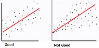
What Does It Look Like?

The simplest explanation I’ve been taught is to picture the overall ‘variance within your variance’.

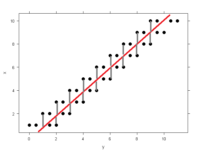
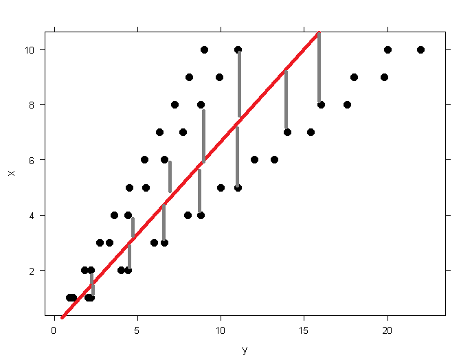
Here are some images generated with R to help frame heteroscedastic patterns vs homoscedastic patterns in your data. In red, you’ll see the result of a hypothetical model, and in grey, the aforementioned residuals. As we trend higher across an independant variable, the residual continues to grow, increasing the estimated statstical error, and decreasing the usefulness of our model.

Scatter	Plots
Homoscedastic	Heteroscedastic
x <- c(1:10)	x <- c(1:10)
y1 <- c(1:10+1)	y1 <- c(1:10*2)
y2 <- c(1:10-1)	y2 <- c(1:10*2.2)
y3 <- c(1:10-0.5)	y3 <- c(1:10*0.9)
y4 <- c(1:10+0.5)	y4 <- c(1:10*1.1)
yT <- c(y1, y2, y3, y4)	yT <- c(y1, y2, y3, y4)
df <- data.frame(x=x, y=yT)	df <- data.frame(x=x, y=yT)
xyplot(y~x,df, par.settings = list(plot.symbol = list(col = “black”, fill = “black”, cex = 2,pch = 20)))	xyplot(x~y,df, par.settings = list(plot.symbol = list(col = “black”, fill = “black”, cex = 2,pch = 20)))