The Great Decider.

The Agenda

Today, let’s focus specifically on the classification portion of the CART set of algorithms, by utilizing SciKit-Learn’s DecicionTreeClassifier module for machine learning solutions.

But first, let’s take a broader look at the concept space and relevant data structures.

Classification and regression trees (CART) Algorithms

CART algorithms are Supervised learning models used for problems involving classification and regression.

Supervised Learning

Supervised learning is an approach for engineering predictive models from known labeled data, meaning the dataset already contains the targets appropriately classed. Our goal is to allow the algorithm to build a model from this known data, to predict future labels (outputs), based on our features (inputs) when introduced to a novel dataset.

Classification Example Problems

1) Identifying fake profiles.

2) Classifying a species.

3) Predicting what sport someone plays.

Classification Tree - Overview

• Objective is to infer class labels from previously unseen data.

• Algorithmically, it is a recursive(divide & conquer) and greedy(favors optimization) solution.

• Is a sequence of if-else questions about features.

• Captures non-linear relationships between features and labels.

• Is non-parametric, based on observed data and does not assume a normal distribution.

• No feature is scaling required.

Classification Model - Approach

Let’s briefly set a mental framework for approaching the creation of a classification model.

Like all things data, we’ll begin with a dataset.

Next, we’ll need to break it into training and test sets.

We can then use the training dataset with a learning algorithm (in our case, the scikit-learn DecisionTreeClassifier module) to create a model via induction, which is then applied to make predictions on the test set of data through deduction.

Here’s a general schematic view of the concept.

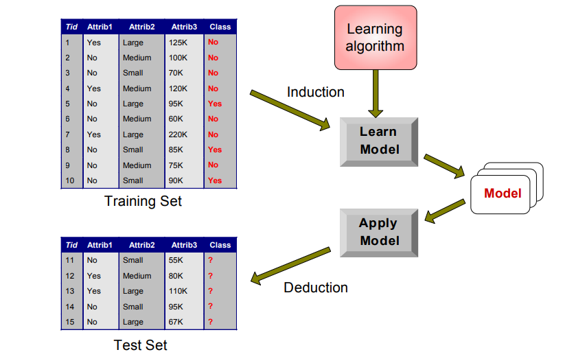
Source: https://www-users.cs.umn.edu/~kumar001/dmbook/dmslides/chap4_basic_classification.pdf

Model Concerns

As powerful as the technique can be, it needs a strong foundation and human-level quality control.

Here are some points to consider as you prepare for your ML task:

A) Are you selecting the right problem to test?

B) Are you capable of supplying sufficient data?

C) Are you providing your model clean data?

D) Are you able to prevent algorithmic biases and confounding factors?

Performance Metrics

It should be noted at the onset, that simple Decision Trees are highly prone to overfitting, leading to models which are difficult to generalize. One method of mitigating this potential risk is to engage in pruning of the tree, i.e., removing parts of the tree which confer no/low power to the model. We will discuss methods of pruning shortly.

A cautious interpretation of seemingly powerful results is encouraged.

Goal: Achieve the highest possible accuracy, while retaining the lowest error rate.

Accuracy Score

• accuracy_score(y_test, y_pred)
  The accuracy score is calculated through the ratio of the correctly predicted data points divided by all predicted data points.

Mean Squared Error

• mean_squared_error(y_test, y_pred)
  Computed average squared difference between the estimated values, and what is being estimated.

Mean Absolute Error

• mean_absolute_error(y_test, y_pred)
  The mean absolute error reflects the magnitude of difference between the prediction and actual.

Score

• score(features, target)
  Mean accuracy on the given test data and labels

Confusion Matrix

• confusion_matrix(y_test, y_pred)
  Summarizes error rate in terms of true/false positives/negatives.

While the rest of the tests outlined above return simple numbers to interpret, the confusion matrix needs a primer on interpetation.

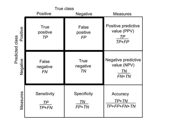
Source: https://bmcgenomics.biomedcentral.com/articles/10.1186/1471-2164-13-S4-S2

Calling confusion_matrix() will yield a result in the form:
[TP,FP]
[FN,TN]

Tree Data Structure - Fundamentals

Reference Image

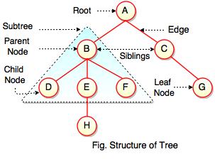
Source: Data Structure Tree Diagram - artbattlesu.com

Unlike common linear data structures, like lists and arrays, a Tree is a non-linear, hierarchical method of storing/modeling data. Visually, you can picture an evolutionary tree, a document object model (DOM) from HTML, or even a flow chart of a company hierarchy.

In contrast to a biological tree originating of kingdom plantae, the data structure tree has a simple anatomy:

A tree consists of nodes and edges.

There are ‘specialized’ node types classified by unique names which represent their place on the hierarchy of the structure.

The root node, is a single point of origin for the rest of the tree. Branches can extend from nodes and link to other nodes, with the link referred to as an edge.

The node which accepts a link/edge, is said to be a child node, and the originating node is the parent.

A single node may have one, two, or no children. If a node has no children, but does have a parent, it is called a leaf. Some will also refer to internal nodes, which have one parent and two children.

Finally, sibling nodes are nodes which share a parent.

Beyond the core anatomy, the tree has unique metrics to be explored: depth and height.

Depth refers to the spatial attributes of an individual node in relation to the root, meaning, how many links/edges are between the specific node and the root node. You could also think of it as the position of the node from root:0 to leaf:m depth.

The height, refers to the number of edges in the longest possible path of the tree, similar to finding the longest carbon chain back in organic chemistry to determine the IUPAC name of the compound.

Decision Tree

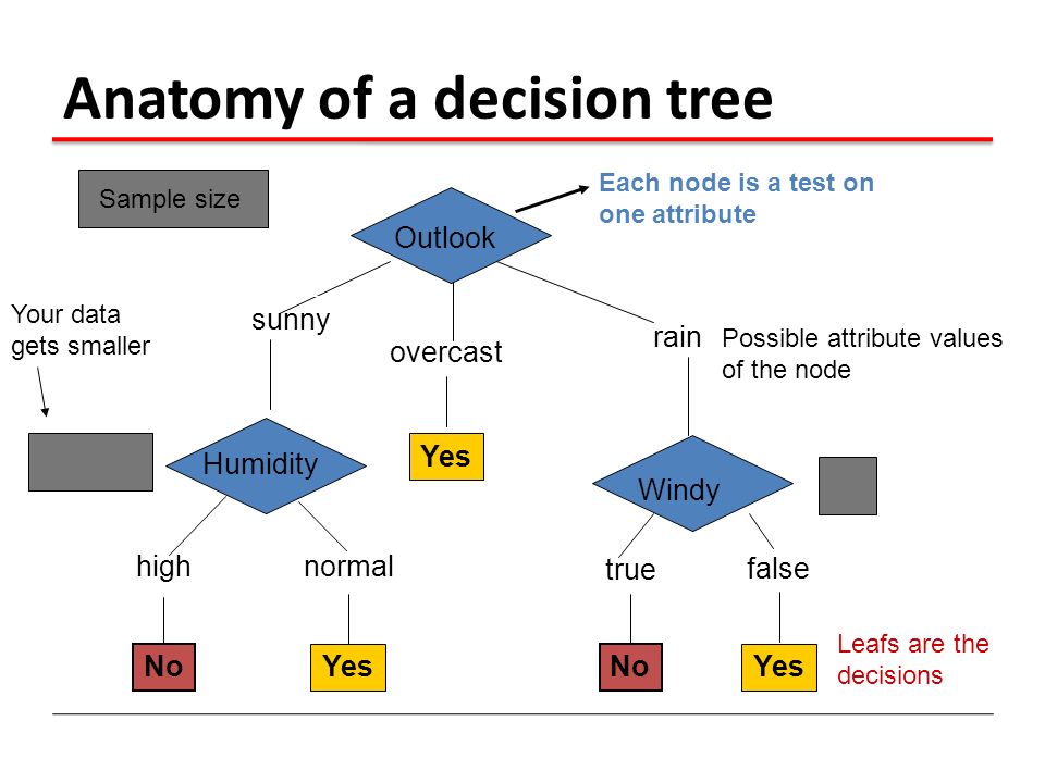
Source: Machine Learning 10601 Recitation 8 Oct 21, 2009 Oznur Tastan

A decision tree, allows us to run a series of if/elif/else tests/questions on a data point, record, or observation with many attributes to be tested. Each node of this tree, would represent some condition of an attribute to test, and the edges/links are the results of this test constrained to some kind of binary decision. An observation travels through each stage, being assayed and partitioned, to reach a leaf node. The leaf contains the final proposed classification.

For example, if we had a dataset with rich features about a human, we could ask many questions about that person and their behavior based on gender(M/F/O), weight(Above/Below a value), height(Above/Below a value), activities(Sets of choices) to make a prediction.

Classification Plot - Simple

Decision Region	Space where instances become assigned to particular class, blue or red, in the plotting space in the diagram.
Decision Boundary	Point of transition from one decision region to another, aka one class/label to another, the diagonal black line.

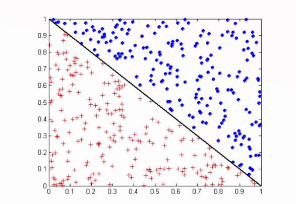
Source: Vipin Kumar CSci 8980 Fall 2002 13 Oblique Decision Trees

Feature Selection

Identification of which features/columns with the highest weights in predictive power.

In our case, the CART algorithm will do the feature selection for us through the Gini Index or Entropy which measure how pure your data is partitioned through it’s journey to a final leaf node classification.

Pruning

As we discussed earlier, decision trees are prone to overfitting. Pruning is one way to mitigate the influence. As each node is a test, and each branch is a result of this test, we can prune unproductive branches which contribute to overfitting. By removing them, we can further generalize the model.

Pre-Pruning

One strategy for pruning is known as pre-pruning. This method relies on ending the series of tests early, stopping the partitioning process. When stopped, what was previously a non-leaf node, becomes the leaf node and a class is declared.

Post-Pruning

Post-Pruning is a different approach. Where pre-pruning occurs during creation of the model, post-pruning begins after the process is complete through the removal of branches. Sets of node removals are tested throughout the branches, to examine the effect on error-rates. If removing particular nodes increases the error-rate, pruning does not occur at those positions. The final tree contains a version of the tree with the lowest expected error-rate.

Decision Tree Classification: Steps to Build and Run

1 Imports

2 Load Data

3 Test and Train Data

4 Instantiate a Decision Tree Classifier

5 Fit data

6 Predict

7 Check Performance Metrics

1 - Import Modules/Libraries [SciKit-Learn]

from sklearn.tree import DecisionTreeClassifier
from sklearn.model_selection import train_test_split
from sklearn.metrics import accuracy_score

2 - Load Data

First, we’re going to want to load a dataset, and create two sets, X and y, which represent our features and our desired label.

# X contains predictors, y holds the classifications
X, y = dataset.data, dataset.target
features = iris.feature_names

3 - Split Dataset into Test and Train sets

Now, we can partition our data into test and train sets, and the typical balance is usually 80/20 or 70/30 test vs train percentages.

The results of the split will be stored in X_train, X_test, y_train, and y_test.

X_train, X_test, y_train, y_test= train_test_split(X, y, test_size=0.2, stratify=y, random_state=1)

4 - Instantiate a DecisionTreeClassifier

We can instantiate our DecisionTreeClassifier object with a max_depth, and a random_state.

random_state allows us a way of ensuring reproducibility, while max_depth is a hyper-parameter, which allows us to control complexity of our tree, but must be used with a cautious awareness. If max_depth is set too high, we risk over-fitting the data, while if it’s too low, we will be underfitting.

dt = DecisionTreeClassifier(max_depth=6, random_state=1)

5 - Fit The Model

We fit our our model by utilizing .fit() and feeding it parameters X_train and y_train which we created previously.

dt.fit(X_train, y_train)

6 - Predict Test Set Labels

We can now test our model by applying it to our X_test variable, and we’ll store this as y_pred.

y_pred = dt.predict(X_test)

7 - Check Performance Metrics

We want to check the accuracy of our model, so let’s run through some performance metrics.

Accuracy Score

def AccuracyCheck(model, X_test, y_pred):
    acc = accuracy_score(y_test, y_pred)
    print('Default Accuracy: {}'.format(round(acc), 3))

Confusion Matrix

def ConfusionMatx(y_test, y_pred):
    print('Confusion Matrix: \n{}'.format(confusion_matrix(y_test, y_pred)))

Mean Absolute Error

def MeanAbsErr(y_test, y_pred):
    mean_err = metrics.mean_absolute_error(y_test, y_pred)
    print('Mean Absolute Error: {}'.format(round(mean_err), 3))

Mean Squared Error

def MeanSqErr(y_test, y_pred):
    SqErr = metrics.mean_squared_error(y_test, y_pred)
    print('Mean Squared Error: {}'.format(round(SqErr), 3))

Score

def DTCScore(X, y, dtc):
    score = dtc.score(X, y, sample_weight=None)
    print('Score: {}'.format(round(score)))

Summary Report
Thanks to the power of Python, we can run all of the tests in one go via scripting:

def MetricReport(X, y, y_test, y_pred, dtc):
    print("Metric Summaries")
    print("-"*16)
    AccuracyCheck(model, X_test, y_pred)
    MeanAbsErr(y_test, y_pred)
    MeanSqErr(y_test, y_pred)
    DTCScore(X, y, dtc)
    ConfusionMatx(y_test, y_pred)
    print("-" * 16)

Hepatitis: A Case Study

We’ll follow the procedures above, with a few twists. We’re going to add a way to visualize our decision tree graph, as well as apply a real dataset using the tools and approaches outlined.

Imports

import pandas as pd
import graphviz
from sklearn import tree
from sklearn.tree import DecisionTreeClassifier
from sklearn.model_selection import train_test_split
from sklearn.metrics import accuracy_score

Dataset

https://archive.ics.uci.edu/ml/datasets/Hepatitis

path = '...hepatitis.csv'
col_names = ['Class', 'Age', 'Sex', 'Steroid', 'Antivirals', 'Fatigue', 'Malaise','Anorexia', 'Liver_Big', 'Liver_Firm',    
             'Spleen_Palp', 'Spiders', 'Ascites', 'Varices', 'Bilirubin', 'Alk_Phosph', 'SGOT', 'Albumin', 'Protime',
             'Histology' ]
csv = pd.read_csv(path, na_values=["?"], names=col_names)
df = pd.DataFrame(csv)

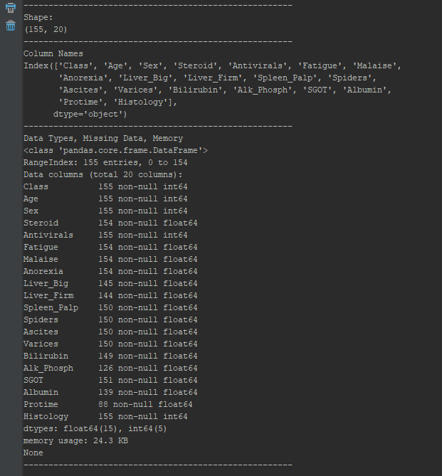
Survey The Data

def minorEDA(df):
    """
    Generates a preliminary EDA Analysis of our file
    args: df - DataFrame of our excel file
    returns: None
    """
    lineBreak = '------------------'
    #Check Shape
    print(lineBreak*3)
    print("Shape:")
    print(df.shape)
    print(lineBreak*3)
    #Check Feature Names
    print("Column Names")
    print(df.columns)
    print(lineBreak*3)
    #Check types, missing, memory
    print("Data Types, Missing Data, Memory")
    print(df.info())
    print(lineBreak*3)

Check Integrity

def check_integrity(input_df):
    """  Check if values missing, generate list of cols with NaN indices
     Args:
             input_df - Dataframe
     Returns:
             List containing column names containing missing data
    """
    if df.isnull().values.any():
        print("\nDetected Missing Data\nAffected Columns:")
        affected_cols = [col for col in input_df.columns if input_df[col].isnull().any()]
        affected_rows = df.isnull().sum()
        missing_list = []
        for each_col in affected_cols:
            missing_list.append(each_col)
        print(missing_list)
        print("\nCounts")
        print(affected_rows)
        print("\n")
        return missing_list
    else:
        pass
    print("\nNo Missing Data Was Detected.")

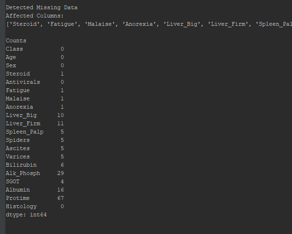
Unfortunately this set contains missing data points, if we don’t clean them up, we’ll recieve an error. To do this, df.dropna(inplace=True) in the __main__ portion of our program will allow us to continue, but our model will ultimately be weaker due to missing inputs.

Set Label Target

def set_target(dataframe, target):
    """
    :param dataframe: Full dataset
    :param target: Name of classification column
    :return x: Predictors dataset
    :return y: Classification dataset
    """
    x = dataframe.drop(target, axis=1)
    y = dataframe[target]
    return x, y

## Decision Tree

 def DecisionTree():
    # Build Decision Tree Classifier
    dtc = DecisionTreeClassifier(max_depth=6, random_state=2)
    return dtc

Test, Train

def TestTrain(X, y):
    """
    :param X: Predictors
    :param y: Classification
    :return: X & Y test/train data
    """
    # Split into training and test set
    X_train, X_test, y_train, y_test = train_test_split(X, y, test_size=0.2, stratify=y, random_state=1)
    return X_train, X_test, y_train, y_test

Fit

def FitData(DTC, X_train, y_train):
    # Fit training data
    return DTC.fit(X_train, y_train)

Predict

def Predict(dtc, test_x):
    y_pred = dtc.predict(test_x)
    return y_pred

Check Accuracy, Metrics, Generate Report

def AccuracyCheck(model, X_test, y_pred):
    #Cneck Accuracy Score
    acc = accuracy_score(y_test, y_pred)
    print('Default Accuracy: {}'.format(round(acc), 3))
    
def ConfusionMatx(y_test, y_pred):
    print('Confusion Matrix: \n{}'.format(confusion_matrix(y_test, y_pred)))

def MeanAbsErr(y_test, y_pred):
    mean_err = metrics.mean_absolute_error(y_test, y_pred)
    print('Mean Absolute Error: {}'.format(round(mean_err), 3))

def MeanSqErr(y_test, y_pred):
    SqErr = metrics.mean_squared_error(y_test, y_pred)
    print('Mean Squared Error: {}'.format(round(SqErr), 3))

def DTCScore(X, y, dtc):
    score = dtc.score(X, y, sample_weight=None)
    print('Score: {}'.format(round(score)))

def MetricReport(X, y, y_test, y_pred, dtc):
    print("Metric Summaries")
    print("-"*16)
    ConfusionMatx(y_test, y_pred)
    MeanAbsErr(y_test, y_pred)
    MeanSqErr(y_test, y_pred)
    DTCScore(X, y, dtc)
    print("-" * 16)    

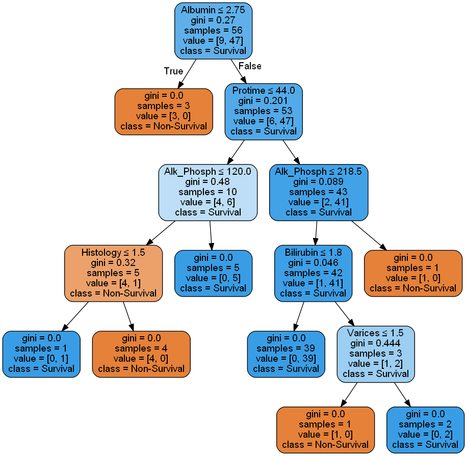
Visualize Tree Graph

def tree_viz(dtc, df, col_names):
    class_n = "Class"
    dot = tree.export_graphviz(dtc, out_file=None, feature_names=col_names, class_names=class_n, filled=True, rounded=True,                                             special_characters=True)
    graph = graphviz.Source(dot)
    graph.format = 'png'
    graph.render('Hep', view=True)

Run

path = 'C:\\Users\\ajh20\\Desktop\\hepatitis.csv'
col_names = ['Class', 'Age', 'Sex', 'Steroid', 'Antivirals', 'Fatigue', 'Malaise','Anorexia', 'Liver_Big', 'Liver_Firm',    
             'Spleen_Palp', 'Spiders', 'Ascites', 'Varices', 'Bilirubin', 'Alk_Phosph', 'SGOT', 'Albumin', 'Protime',
             'Histology' ]
csv = pd.read_csv(path, na_values=["?"], names=col_names)
df = pd.DataFrame(csv)
minorEDA(df)
check_integrity(df)
df.dropna(inplace=True)
X, y = set_target(df, 'Class')
dtc = DecisionTree()
X_train, X_test, y_train, y_test = TestTrain(X, y)
model_test = FitData(dtc, X_train, y_train)
y_pred = Predict(dtc, X_test)
AccuracyCheck(model_test, X_test, y_pred)
tree_viz(dtc, df, col_names)

All-In-One

import pandas as pd
import graphviz
from sklearn import tree
from sklearn.tree import DecisionTreeClassifier
from sklearn.model_selection import train_test_split
from sklearn.metrics import accuracy_score


def set_target(dataframe, target):
    """
    :param dataframe: Full dataset
    :param target: Name of classification column
    :return x: Predictors dataset
    :return y: Classification dataset
    """
    x = dataframe.drop(target, axis=1)
    y = dataframe[target]
    return x, y


def TestTrain(X, y):
    """
    :param X: Predictors
    :param y: Classification
    :return: X & Y test/train data
    """
    # Split into training and test set
    X_train, X_test, y_train, y_test = train_test_split(X, y, test_size=0.2, stratify=y, random_state=1)
    return X_train, X_test, y_train, y_test


def DecisionTree():
    # Build Decision Tree Classifier
    dtc = DecisionTreeClassifier(max_depth=6, random_state=2)
    return dtc


def FitData(DTC, X_train, y_train):
    # Fit training data
    return DTC.fit(X_train, y_train)


def Predict(dtc, test_x):
    y_pred = dtc.predict(test_x)
    return y_pred


def AccuracyCheck(model, X_test, y_pred):
    #Cneck Accuracy Score
    acc = accuracy_score(y_test, y_pred)
    print('Default Accuracy: {}'.format(round(acc), 3))


def ConfusionMatx(y_test, y_pred):
    print('Confusion Matrix: \n{}'.format(confusion_matrix(y_test, y_pred)))


def MeanAbsErr(y_test, y_pred):
    mean_err = metrics.mean_absolute_error(y_test, y_pred)
    print('Mean Absolute Error: {}'.format(round(mean_err), 3))


def MeanSqErr(y_test, y_pred):
    SqErr = metrics.mean_squared_error(y_test, y_pred)
    print('Mean Squared Error: {}'.format(round(SqErr), 3))


def DTCScore(X, y, dtc):
    score = dtc.score(X, y, sample_weight=None)
    print('Score: {}'.format(round(score)))


def MetricReport(X, y, y_test, y_pred, dtc):
    print("Metric Summaries")
    print("-"*16)
    ConfusionMatx(y_test, y_pred)
    MeanAbsErr(y_test, y_pred)
    MeanSqErr(y_test, y_pred)
    DTCScore(X, y, dtc)
    print("-" * 16)


def tree_viz(dtc, df, col_names):
    class_n = ['0','1']
    dot = tree.export_graphviz(dtc, out_file=None, feature_names=col_names, class_names=class_n, filled=True, rounded=True,       
                               special_characters=True)
    graph = graphviz.Source(dot)
    graph.format = 'png'
    graph.render('Hep', view=True)


def minorEDA(df):
    """
    Generates a preliminary EDA Analysis of our file

    args: df - DataFrame of our excel file
    returns: None
    """
    lineBreak = '------------------'
    #Check Shape
    print(lineBreak*3)
    print("Shape:")
    print(df.shape)
    print(lineBreak*3)
    #Check Feature Names
    print("Column Names")
    print(df.columns)
    print(lineBreak*3)
    #Check types, missing, memory
    print("Data Types, Missing Data, Memory")
    print(df.info())
    print(lineBreak*3)


def check_integrity(input_df):
    """  Check if values missing, generate list of cols with NaN indices
     Args:
             input_df - Dataframe
     Returns:
             List containing column names containing missing data
    """
    if df.isnull().values.any():
        print("\nDetected Missing Data\nAffected Columns:")
        affected_cols = [col for col in input_df.columns if input_df[col].isnull().any()]
        affected_rows = df.isnull().sum()
        missing_list = []
        for each_col in affected_cols:
            missing_list.append(each_col)
        print(missing_list)
        print("\nCounts")
        print(affected_rows)
        print("\n")
        return missing_list
    else:
        pass
    print("\nNo Missing Data Was Detected.")


path = 'C:\\Users\\ajh20\\Desktop\\hepatitis.csv'
col_names = ['Class', 'Age', 'Sex', 'Steroid', 'Antivirals', 'Fatigue', 'Malaise','Anorexia', 'Liver_Big', 'Liver_Firm',
             'Spleen_Palp', 'Spiders', 'Ascites', 'Varices', 'Bilirubin', 'Alk_Phosph', 'SGOT', 'Albumin', 'Protime',
             'Histology' ]
csv = pd.read_csv(path, na_values=["?"], names=col_names)
df = pd.DataFrame(csv)
minorEDA(df)
check_integrity(df)
df.dropna(inplace=True)
X, y = set_target(df, 'Class')
dtc = DecisionTree()
X_train, X_test, y_train, y_test = TestTrain(X, y)
model_test = FitData(dtc, X_train, y_train)
y_pred = Predict(dtc, X_test)
AccuracyCheck(model_test, X_test, y_pred)
tree_viz(dtc, df, col_names)