It’s Getting Hot In Here.

Let’s revisit a previous post, where we had been working with Abalone data from the UCI Machine Learning Repository.

Previously, we had generated a scatter matrix to look for linear correlations, here’s a refresher of our results:

Scatter Matrix - Abalone Data

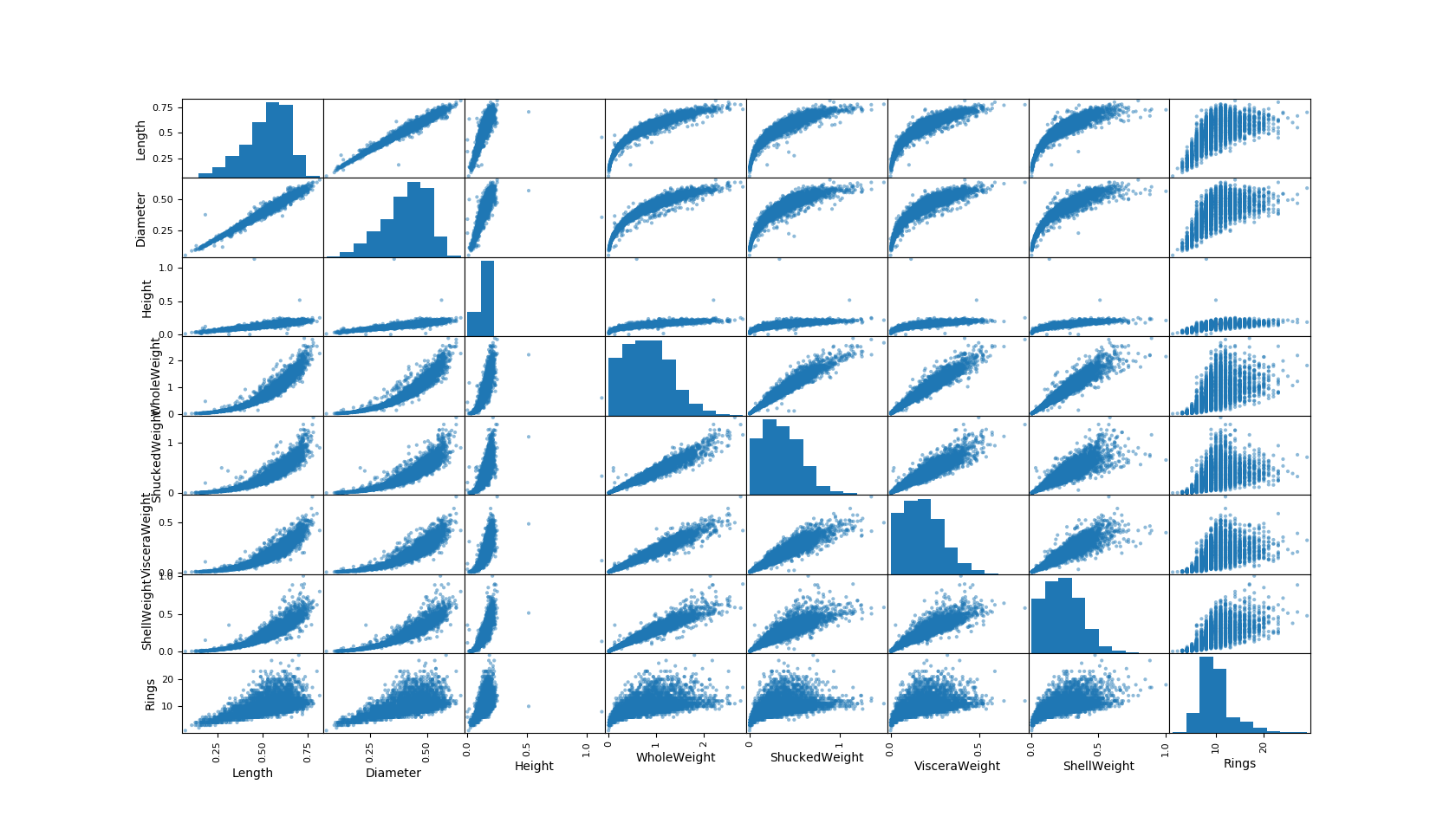
This time, let’s use the same dataset to generate a Seaborn Heat Map of correlation coefficients.

We’ll be utilizing the following Python modules

Imports

import pandas as pd
import matplotlib.pyplot as plt
import seaborn as sns

I’ve modularized the previous data call, which will give us a Pandas DataFrame of the online data.

Grab All The Data

def getDF(data_url, columns):
    #retrieve data from url, create dataframe, return it
    data = pd.read_csv(data_url, names=columns)
    return data

Next, let’s build our heat map! It’s important to note that we will be creating our own color gradient map, with high correlations displayed in increasing red shades, and lower correlations trending into the blue hues.

We will also add our correlation values inside the graph itself, displaying floating numbers in each category.

Seaborn Heat Map

def heatMap(df):
    #Create Correlation df
    corr = df.corr()
    #Plot figsize
    fig, ax = plt.subplots(figsize=(10, 10))
    #Generate Color Map
    colormap = sns.diverging_palette(220, 10, as_cmap=True)
    #Generate Heat Map, allow annotations and place floats in map
    sns.heatmap(corr, cmap=colormap, annot=True, fmt=".2f")
    #Apply xticks
    plt.xticks(range(len(corr.columns)), corr.columns);
    #Apply yticks
    plt.yticks(range(len(corr.columns)), corr.columns)
    #show plot
    plt.show()

Visualize It

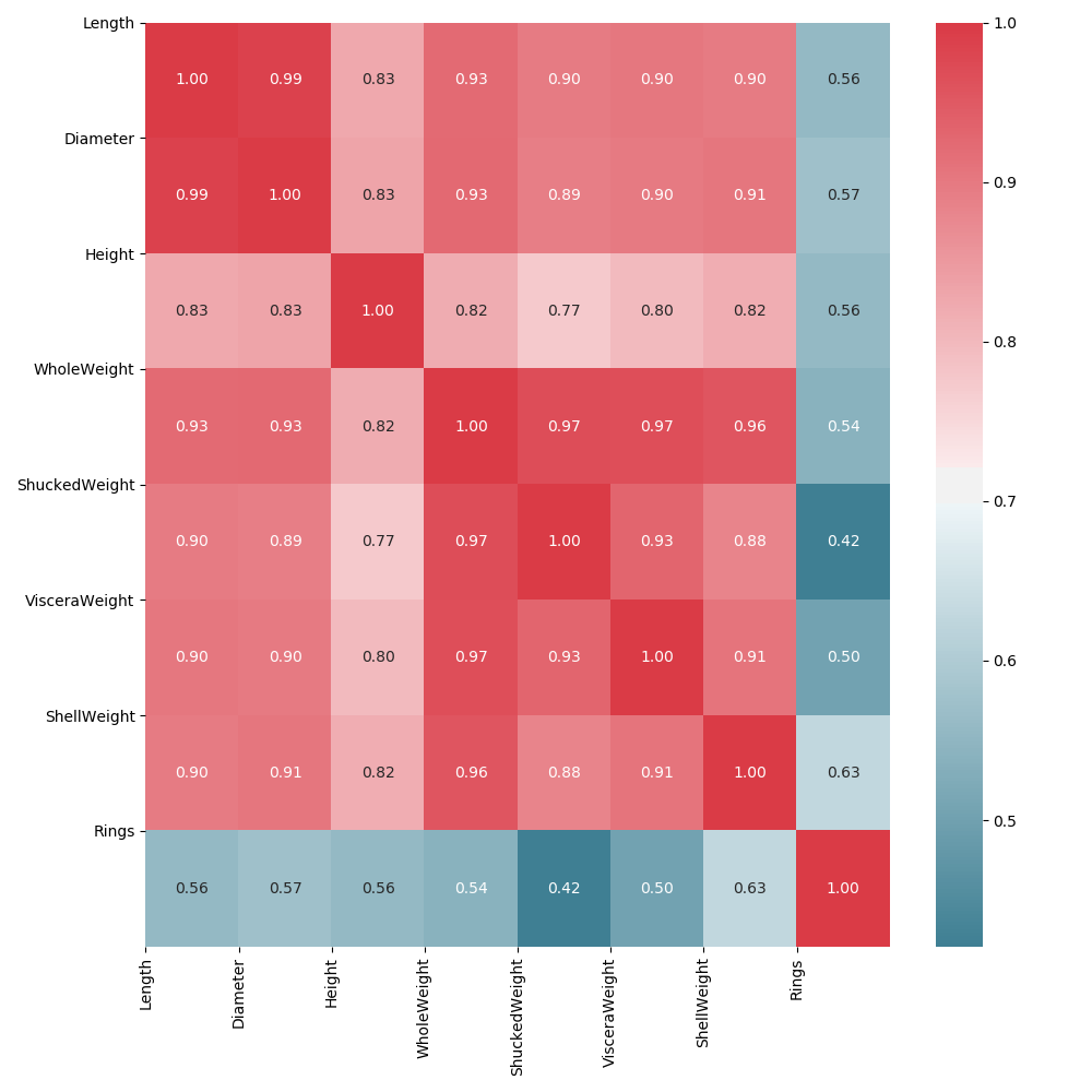
Awesome! However, we can do better. The diagonal plane mirrors itself on either side, with both redundant results AND self to self correlations, which we should drop.

Toggling Our Plot, Apply Mask Parameter

Let’s alter our previous code a little, by adding in a ‘mirror’ parameter that will allow us to drop our redundant mappings.

If the user enters a second paramenter, ‘mirror’, as ‘False’, we will generate half the visualization as we did previously.

def heatMap(df, mirror):

   # Create Correlation df
   corr = df.corr()
   # Plot figsize
   fig, ax = plt.subplots(figsize=(10, 10))
   # Generate Color Map
   colormap = sns.diverging_palette(220, 10, as_cmap=True)
   
   if mirror == True:
      #Generate Heat Map, allow annotations and place floats in map
      sns.heatmap(corr, cmap=colormap, annot=True, fmt=".2f")
      #Apply xticks
      plt.xticks(range(len(corr.columns)), corr.columns);
      #Apply yticks
      plt.yticks(range(len(corr.columns)), corr.columns)
      #show plot

   else:
      # Drop self-correlations
      dropSelf = np.zeros_like(corr)
      dropSelf[np.triu_indices_from(dropSelf)] = True
      # Generate Color Map
      colormap = sns.diverging_palette(220, 10, as_cmap=True)
      # Generate Heat Map, allow annotations and place floats in map
      sns.heatmap(corr, cmap=colormap, annot=True, fmt=".2f", mask=dropSelf)
      # Apply xticks
      plt.xticks(range(len(corr.columns)), corr.columns);
      # Apply yticks
      plt.yticks(range(len(corr.columns)), corr.columns)
   # show plot
   plt.show()
   

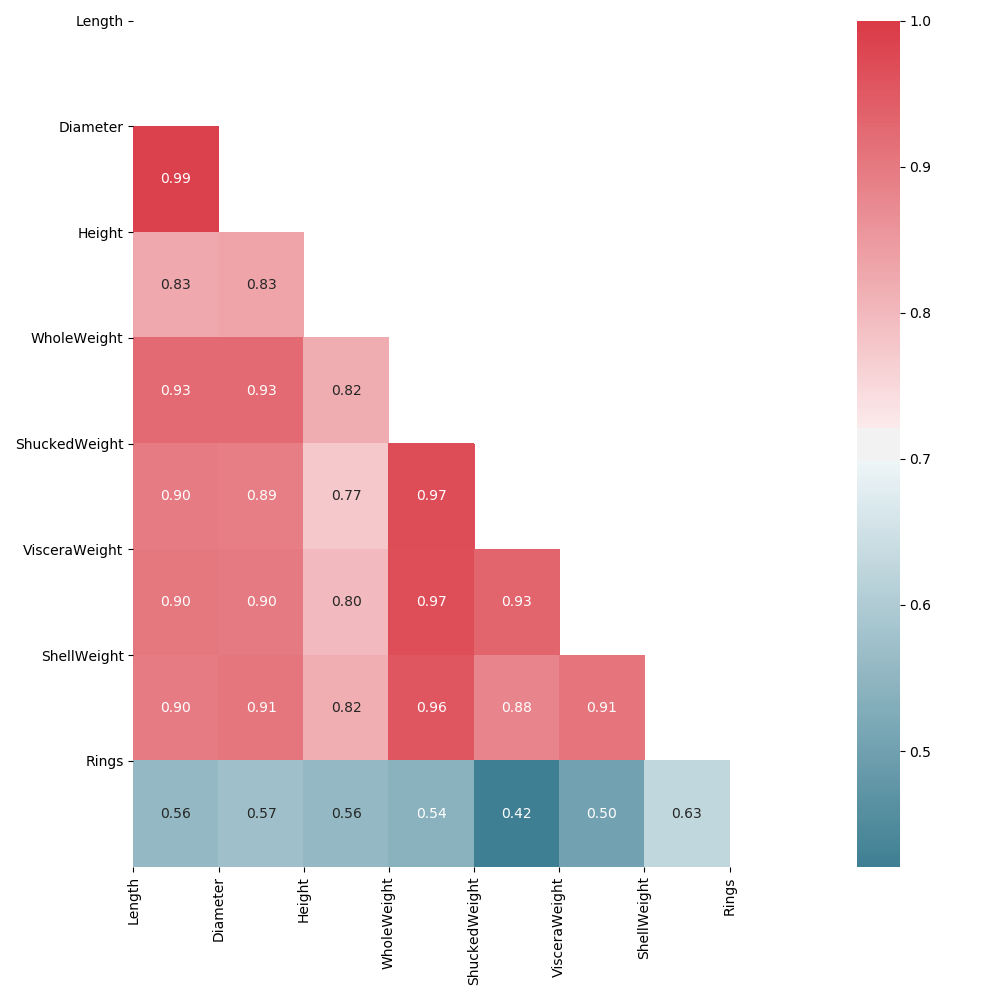
Much better! We’ve dropped a substantial amount of redundant information that only served to act as distractive noise. Now we can focus on the relationships with ease.

Code Summary

Part I

import pandas as pd
import matplotlib.pyplot as plt
import seaborn as sns

def getDF(data_url, columns):
    #retrieve data from url, create dataframe, return it
    data = pd.read_csv(data_url, names=columns)
    return data
    
    def heatMap(df):
    #Create Correlation df
    corr = df.corr()
    #Plot figsize
    fig, ax = plt.subplots(figsize=(10, 10))
    #Generate Color Map
    colormap = sns.diverging_palette(220, 10, as_cmap=True)
    #Generate Heat Map, allow annotations and place floats in map
    sns.heatmap(corr, cmap=colormap, annot=True, fmt=".2f")
    #Apply xticks
    plt.xticks(range(len(corr.columns)), corr.columns);
    #Apply yticks
    plt.yticks(range(len(corr.columns)), corr.columns)
    #show plot
    plt.show()

Part II

    def halfHeatMap(df, mirror):

       # Create Correlation df
       corr = df.corr()
       # Plot figsize
       fig, ax = plt.subplots(figsize=(10, 10))
       # Generate Color Map
       colormap = sns.diverging_palette(220, 10, as_cmap=True)

       if mirror == True:
          #Generate Heat Map, allow annotations and place floats in map
          sns.heatmap(corr, cmap=colormap, annot=True, fmt=".2f")
          #Apply xticks
          plt.xticks(range(len(corr.columns)), corr.columns);
          #Apply yticks
          plt.yticks(range(len(corr.columns)), corr.columns)
          #show plot

       else:
          # Drop self-correlations
          dropSelf = np.zeros_like(corr)
          dropSelf[np.triu_indices_from(dropSelf)] = True
          # Generate Color Map
          colormap = sns.diverging_palette(220, 10, as_cmap=True)
          # Generate Heat Map, allow annotations and place floats in map
          sns.heatmap(corr, cmap=colormap, annot=True, fmt=".2f", mask=dropSelf)
          # Apply xticks
          plt.xticks(range(len(corr.columns)), corr.columns);
          # Apply yticks
          plt.yticks(range(len(corr.columns)), corr.columns)
       # show plot
       plt.show()