Your data will be good to you, if you’re good to it. Be responsible, use Pandas.

Loading Data:

First, you’ll need to import the library, using the keyword ‘as’ allows us to reference the library by simply using pd as a way to call a feature in Pandas. Ex. pd.value_counts()

import pandas as pd

Now, we can use the feature read_csv() to construct a call to the file that contains our data.

raw = pd.read_csv('filepath/filename.csv')

Great!

That was easy, but it won’t always be easy. Your file may have an improper format at the initial read-state, but we can remedy this with available attributes we can define in the .read_csv call.

pandas.read_csv(filepath_or_buffer, sep=', ', delimiter=None, header='infer', names=None, index_col=None, usecols=None, squeeze=False, prefix=None, mangle_dupe_cols=True, dtype=None, engine=None, converters=None, true_values=None, false_values=None, skipinitialspace=False, skiprows=None, skipfooter=None, nrows=None, na_values=None, keep_default_na=True, na_filter=True, verbose=False, skip_blank_lines=True, parse_dates=False, infer_datetime_format=False, keep_date_col=False, date_parser=None, dayfirst=False, iterator=False, chunksize=None, compression='infer', thousands=None, decimal='.', lineterminator=None, quotechar='"', quoting=0, escapechar=None, comment=None, encoding=None, dialect=None, tupleize_cols=False, error_bad_lines=True, warn_bad_lines=True, skip_footer=0, doublequote=True, delim_whitespace=False, as_recarray=False, compact_ints=False, use_unsigned=False, low_memory=True, buffer_lines=None, memory_map=False, float_precision=None)

…it’s a lot to take in this early, so we’ll focus on the most common of that long list we would likely find useful.

sep - Defines the seperator between values, example, ,

encoding - Defines the encoding, example UTF8 vs Latin1

skiprows - Sets line numbers to skip, or number of lines to skip, ex = [0:2]

date_parser - Converts strings to an array of datetime instances

We can string them together like you’d expect:

pd.read_csv('filepath/filename.csv', sep = ',', encoding = 'UTF-8', skiprows[1]

Moving on.

Since we’re using Pandas and working with data, you should be excited to utilize a DataFrame, a Pythonic version of the same structure from R. These are wildly useful for every stage of analysis. We will call pd.DataFrame() to produce our desired structure, which we’ll store as df.

df = pd.DataFrame(raw)

Data Exploration - BitCoin Market Value History

Those few steps have allowed us to gather immediate knowledge about our data, and perhaps even our problem we’re trying to solve.

Pandas has many native features for data exploration, and we’ll cover the most common of which you’ll almost always want to use when you are working with a new set of information.

.head() - Returns the observations and variables of top level subset of your dataframe

.tail() - Returns the observations and variables of bottom level subset of your dataframe

.describe() - Summary of your statistics (min/max, mean, quartiles, standard dev…)

.info() - Summary of your dataframe, returns information about datatypes (obj vs int etc)

.shape - Returns the count of rows and columns

value_counts() - Returns counts of variables and observations (Ex. How many observations for Male vs Female categories respectively)

You’ll likely be familiar with most of these if you’ve used R, many of Pandas’ features reproduce the features of R in a more OOP/scriptable/friendly manner.

Let’s look at some example implementations for our dataset.

print(pd.shape(df))

(1609, 7)

print(df.info())

<class 'pandas.core.frame.DataFrame'>
RangeIndex: 1609 entries, 0 to 1608
Data columns (total 7 columns):
Date          1609 non-null object
Open          1609 non-null float64
High          1609 non-null float64
Low           1609 non-null float64
Close         1609 non-null float64
Volume        1609 non-null object
Market Cap    1609 non-null object
dtypes: float64(4), object(3)
memory usage: 69.2+ KB

It looks like we’ll need to clean up ‘Volume’ and ‘Market Cap’, both are stored as objects, when we’d probably get the most value out of them if they were stored as float64 as in the case of the other numeric categories.

print(df.head())

           Date     Open     High      Low    Close         Volume  \
0  Sep 22, 2017  3628.02  3758.27  3553.53  3630.70  1,194,830,000   
1  Sep 21, 2017  3901.47  3916.42  3613.63  3631.04  1,411,480,000   
2  Sep 20, 2017  3916.36  4031.39  3857.73  3905.95  1,213,830,000   
3  Sep 19, 2017  4073.79  4094.07  3868.87  3924.97  1,563,980,000   
4  Sep 18, 2017  3591.09  4079.23  3591.09  4065.20  1,943,210,000   

       Market Cap  
0  60,152,300,000  
1  64,677,600,000  
2  64,918,500,000  
3  67,520,300,000  
4  59,514,100,000  

print(df.tail())

 Date    Open    High     Low   Close Volume     Market Cap
1604  May 02, 2013  116.38  125.60   92.28  105.21      -  1,292,190,000
1605  May 01, 2013  139.00  139.89  107.72  116.99      -  1,542,820,000
1606  Apr 30, 2013  144.00  146.93  134.05  139.00      -  1,597,780,000
1607  Apr 29, 2013  134.44  147.49  134.00  144.54      -  1,491,160,000
1608  Apr 28, 2013  135.30  135.98  132.10  134.21      -  1,500,520,000

print(df['Close'].value_counts())

104.00     4
111.50     3
236.15     3
129.00     3
249.01     2

Here, we took a count of the top 5 repeating Closing values of BitCoin, all of which occurred relatively early in the life of the currency.

print(df.describe())

              Open         High          Low        Close
count  1609.000000  1609.000000  1609.000000  1609.000000
mean    693.497433   712.776582   674.365525   695.563356
std     797.365059   825.622752   768.109415   800.557569
min      68.500000    74.560000    65.530000    68.430000
25%     260.720000   265.610000   254.200000   260.890000
50%     446.890000   452.480000   440.500000   447.530000
75%     701.340000   714.120000   670.880000   702.030000
max    4901.420000  4975.040000  4678.530000  4892.010000

We should also briefly introduce plotting with Pandas, which we’ll primarily approach through MatPlotLab, it’s great to get a visualization of your data as you explore. We’ll look at the ‘Highs’ of the currency over time with frequency.

First, import matplotlib

import matplotlib.pyplot as plt

Then, select the column you want to assay, ‘High’, and the type of plot, a histogram, passed as ‘hist’

df.High.plot('hist')

Now, we want to add labels:

plt.xlabel('Highs')

plt.ylabel('Observations')

And a title:

plt.title('BitCoin Market Value - Highs')

Finally, we generate the plot with:

plt.show()

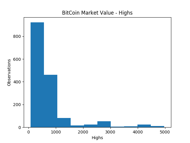
Easy! BUT it’s not a good way to parse and display this data!

We’d much rather look at a timeseries representation using a lineplot. We’ll repeat much of the same code, but with some important alterations:

We’re going to manually set the X and Y values

df.plot(kind = 'line', x = 'Date', y = 'High')

Correct our labels

plt.xlabel('Date')

plt.ylabel('High')

Extend our title

plt.title('BitCoin Market Value Over Time')

And once again, show the plot

plt.show()

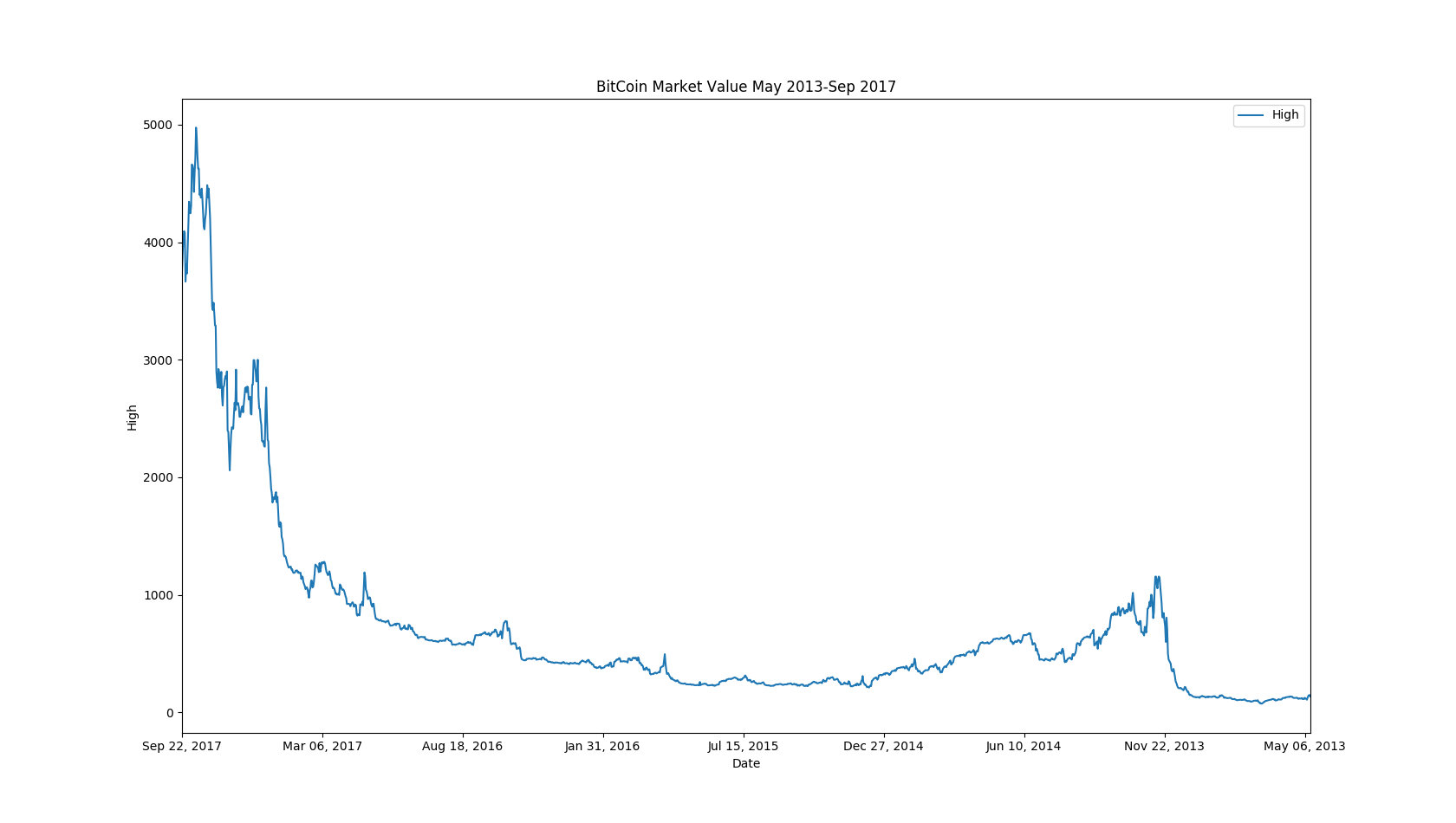
Better!

BUT, I’M NOT HAPPY, YET…

We want our graphs to be intuitive, to communicate enough information without our own commentary. If you weren’t paying attention to the axes, you might think the value of BitCoin has gone down with time. The problem is that the .csv file has the dates stored in descending order, so our graph is reflected from our ideal vision.

We can remedy this!

Let’s reverse our data frame using the .iloc[start:stop:step] model

reversed_df = df.iloc[::-1]

[::-1] means we are going to move each element in our dataframe back a position, effectively reversing the entire thing!

Now, we can proceed exactly as before with the corrected data source:

reversed_df.plot(kind = 'line', x = 'Date', y = 'High')

plt.xlabel('Date')

plt.ylabel('High')

plt.title('BitCoin Market Value May 2013-Sep 2017')

plt.show()

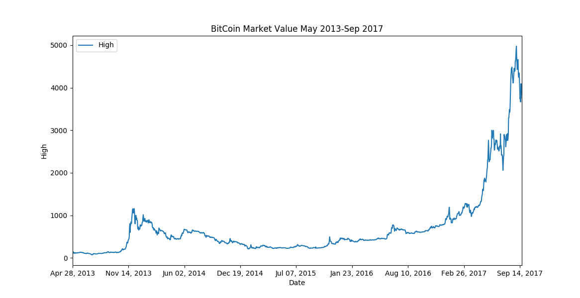
Finally, we can all regret not jumping into the explosive opportunity, much, much earlier!

In just a few short years, the value of the cryptocurrency has shot up from less than $100 to almost $5000 (and if you’re following it now, it’s even higher!

It’s important to explore your data early, you’ll avoid some common problems(improper datatypes, missing values, improper naming conventions, duplicate data, and many more), and it’s just the proper thing to do. As you explore your data, you can be quite productive. The summary statistics alone are worth your time, but you’ll also be developing a knowledge of potential problems; both pre-existing and those down the line. You’re taking the first step towards the cleaning stage of the data science process.

.DataFrame

We have seemingly limitless control over our data when it’s structured in a DataFrame. Slicing, rotating, renaming, refactoring, plotting, insertion and extraction; you can do it all.