Mobile Game AB Testing

We’ve talked about AB testing in an earlier post, now is the time to give a full-spectrum run through a real dataset courtesy
of DataCamp.
The fine folks at DataCamp released a project for AB testers to play with focused around data from a game called Cookie Cats. I highly recommend any data-curious people, from novice to experienced, to give their service a shot.
Today’s project is centered around AB testing in mobile games development, we’re going to model the base DataCamp work flow while adding our own twists and approaches as we proceed.
Let’s begin by importing our libraries and data, and seeing what we have to work with!
IMPORT LIBRARIES
# Importing pandas
import pandas as pd
import matplotlib.pyplot as plt
Now the data…
READ DATA
# Reading in the data
df = pd.read_csv("datasets/cookie_cats.csv")
Great! So, let’s start our investigation.
EDA
# Check Head
#print(df.head())

# Integrity Check
#df.info()

# Describe
#df.describe()

# Check levels
df.version.unique()
EDA OUTPUT:
   userid  version  sum_gamerounds  retention_1  retention_7
0     116  gate_30               3        False        False
1     337  gate_30              38         True        False
2     377  gate_40             165         True        False
3     483  gate_40               1        False        False
4     488  gate_40             179         True         True

<class 'pandas.core.frame.DataFrame'>
RangeIndex: 90189 entries, 0 to 90188
Data columns (total 5 columns):
userid            90189 non-null int64
version           90189 non-null object
sum_gamerounds    90189 non-null int64
retention_1       90189 non-null bool
retention_7       90189 non-null bool
dtypes: bool(2), int64(2), object(1)
memory usage: 2.2+ MB

userid	sum_gamerounds
count	9.018900e+04	90189.000000
mean	4.998412e+06	51.872457
std	2.883286e+06	195.050858
min	1.160000e+02	0.000000
25%	2.512230e+06	5.000000
50%	4.995815e+06	16.000000
75%	7.496452e+06	51.000000
max	9.999861e+06	49854.000000

array(['gate_30', 'gate_40'], dtype=object)
Output Summary:
It appears that we have 90,189 rows populated over 5 columns, and no missing data! Perfect.
Our columns are userid, version, sum_gamerounds, retention_1, and retention_7. Only two columns contain
numeric variables, userid and sum_gamerounds. Userid reflects unique user ID’s, and sum_gamerounds reflects the number
of rounds played by each unique user. Version contains 2 groups, and will be the source of some of our AB groupings. As we
see from our EDA output, there are two levels, gate_30 and gate_40. Finally, our last two columns, retention_1 and
retention_7 are boolean values, True or False, indicating whether a player is still active after 1 or 7 days.
Like most “free” mobile games, there is an economic element for the craftsmen of the product to generate revenue. In this case,
there is a forced cool-down period after so many levels, which the player can remove by paying a fee. The version column
in our dataframe reflects versions with different gates preventing the player’s progress, after 30 levels or after 40, these
are recorded as gate_30 and gate_40.
These two versions allow us a fine entry point to AB testing.
Sample Size
Let’s first define the population sizes we’re dealing with to make sure we can proceed with a statistically sound comparison.
# Counting the number of players in each AB group.
A = df.version.groupby(df.version == "gate_30").count()
B = df.version.groupby(df.version == "gate_40").count()
print(A)
print(B)
Output:
` version False 45489 True 44700 Name: version, dtype: int64
version False 44700 True 45489 Name: version, dtype: int64 `
Of our 90,189 total records, approximately half are using version gate_30 (which we will call Group A) and the other half are using version gate_40 (which we will call version B).
This is great, we can proceed with the analysis.
How Much Do They Play?
We want to see how many how long players typically stay with a product. One way to measure the metric in this case, is to examine how many rounds each user plays.
Since we’re using a Pandas DataFrame, we can take the following approach. We’ll use .groupby() to set each user’s experience
to a bin, and return a total count. We’ll then plot how many players are active within a set range, showing us the counts of
players within the 0-100 range of total rounds played.
# Counting the number of players for each number of gamerounds
plot_df = df.groupby("sum_gamerounds").count()

# Plotting the distribution of players that played 0 to 100 game rounds
ax = plot_df[:100].plot()
ax.set_xlabel("Total Game Rounds")
ax.set_ylabel("userid")
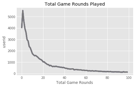
Conclusion:
It appears that the vast majority of users are playing less than 20 rounds in total, over the recording of this data.
Let’s take the same approach to see if there is much of a difference in the number of games played in our AB versions allotted to each user.
Group Distributions: A vs B Total Plays
Set-Up
This time, we’ll need to massage the data a bit more. We’re also going to switch to an overlayed bar-plot of the distinct AB group distributions.
Since we’ve already identified that the drop off in users occurs in less than 20 sessions, let’s also change our bin distribution to get a more nuanced view of the low end and high end of user activities.
plt.style.use('ggplot')

# Counting the number of players for each number of gamerounds
Group_A = df[df.version == 'gate_30']
print(Group_A.head())
print(Group_B.head())
Group_B = df[df.version == 'gate_40']
bins = [0,1,10,20,30,40,50,60,70,80,90,100,200,500]
plot_GA = pd.DataFrame(Group_A.groupby(pd.cut(Group_A["sum_gamerounds"], bins=bins)).count())
plot_GB = pd.DataFrame(Group_B.groupby(pd.cut(Group_B["sum_gamerounds"], bins=bins)).count())
Plot It!
Remember, we’re going to overlay our graphs, so take particular notice of one approach that works
for our example, where we assign the second graph the parameter ax=ax to allow the overlay of the second distribution.
# Plotting the distribution of players that played 0 to 100 game rounds
ax = plot_GA[:50].plot(kind = 'bar', y="userid", color = "black", alpha = 1,
                       title = 'Total Usage By Groups')
plot_GB[:50].plot(kind = 'bar', y="userid", ax=ax, color = "red", alpha = 0.7 )
ax.set_xlabel("Total Game Rounds")
ax.set_ylabel("Players")
#plt.axvline(30, linestyle='dashed', linewidth=2)
#plt.axvline(40, linestyle='dashed', linewidth=2)
plt.legend(["Group A", "Group B"])
plt.tight_layout()
plt.grid(True)
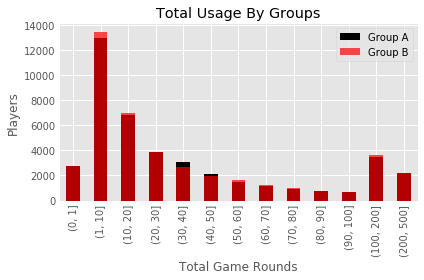
There doesn’t seem to be a large difference between the two versions overall. However, there does seem to be some slight disparities around the 30-40 marks that may be related to the AB test at hand.
Please Come Back
Another metric we can use to guage the success of the product, is in the capture of returning users. If our revenue model is based on users, we don’t want them to give up on us early. Let’s look at how many players come back the day after installing the game.
# Calculate percent of returning users - next day
oneday = df.retention_1.sum()/df.retention_1.count()
print(str(oneday*100)+"%")
Output:
44.52% Return the day following an installation of the product.
Slightly less than half? Ok, just out of curiousity is there any fundamental difference in our two user populations from the start regardless of version impact? This time, let’s do as we did above, but this time group them by version group and see how the numbers pan out.
# Calculating 1-day retention for each AB-group
oneday = df.retention_1.groupby(df.version).sum()/df.retention_1.groupby(df.version).count()
print(oneday)
Output:
gate_30 44.818792
gate_40 44.228275
It looks like regardless of version, next day returns are essentially the same between our experimental groups.
But, there IS that 0.6% loss in return players randomized to the 40 round gate…could it be significant? Maybe this product will see millions of users and that extra 0.6% could translate into some paying customers and/or ad dollars.
It’s worth investigating.
We can use Bootstrapping to test our confidence. Bootstrapping is used in many disciplines, such as in molecular
biology to help the analysis of phylogenetics, to re-sample and replace data to and test our statistical confidence in our
results.
Bootstrapping Means - Sampling
# Creating an list with bootstrapped means for each AB-group
boot_1d = []
for i in range(500):
    boot_mean = df.retention_1.sample(frac=1, replace=True).groupby(df.version).mean()
    boot_1d.append(boot_mean)

# Transforming the list to a DataFrame
boot_1d = pd.DataFrame(boot_1d)
print(boot_1d)

# A Kernel Density Estimate plot of the bootstrap distributions
boot_1d.plot.kde()
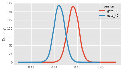
Calculating AB Group Percent Differences For A New Column, and Plotting
# Populate a new % Difference Column
boot_1d['difference'] = (boot_1d['gate_30'] - boot_1d['gate_40']) /  boot_1d['gate_40'] * 100

# Plot the new Column
ax = boot_1d['difference'].plot.kde()
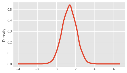
Calculating the probability that 1-day retention is greater when the gate is at level 30
prob = (boot_1d['diff'] > 0).sum() / len(boot_1d['diff'])
print(str(prob*100)+"%")
Output:
96.26%
Calculating 7-day retention for both AB-groups
sevenday = df.retention_7.sum()/df.retention_7.count()
print(sevenday)
Output:
0.186064819435
Creating a list with bootstrapped means for each AB-group
boot_7d = []
for i in range(500):
boot_mean = df.retention_7.sample(frac=1, replace=True).groupby(df.version).mean()
boot_7d.append(boot_mean)
# Transforming the list to a DataFrame
boot_7d = pd.DataFrame(boot_7d)
# Adding a column with the % difference between the two AB-groups
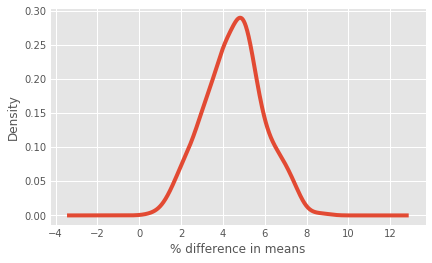
boot_7d['diff'] = (boot_7d['gate_30'] - boot_7d['gate_40']) / boot_7d['gate_40'] * 100
# Plotting the bootstrap % difference
ax = boot_7d['diff'].plot.kde()
ax.set_xlabel("% difference in means")

# Calculating the probability that 7-day retention is greater when the gate is at level 30
prob = (boot_7d['diff'] > 0).sum() / len(boot_7d['diff'])

# Pretty printing the probability
print(prob)